Fundamentals of Ohmic Networks, Linear Circuit Theorems & Solid-State Biasing
Published by the Electrical Engineering & Applied Physics Guild • Standards Compliant with IEEE 315, IEC 60062, and EIA-RS-279A.
1. The Electromagnetic Basis of Ohm's and Joule's Laws
Formulated in 1827 by Bavarian physicist Georg Simon Ohm in his seminal treatise Die galvanische Kette, mathematisch bearbeitet, Ohm's Law establishes the macroscopic constitutive relationship governing electric charge carriers drifting through a conductive lattice under an applied electrostatic potential gradient. Microscopically, according to the classical Drude model of electron transport, mobile conduction electrons undergo stochastic momentum-relaxing collisions with vibrating atomic ion cores, characterized by a mean free time between collisions τ. The resulting steady-state drift velocity is directly proportional to the applied electric field:
where J is current density (A/m²), σ is macroscopic electrical conductivity (S/m), n is electron volume density, and m_e is effective electron mass. Integrating this microscopic field equation across a cylindrical conductor of uniform cross-sectional area A and length L yields the macroscopic relation V = I × R, where bulk resistance R = ρ × L / A, with ρ = 1/σ denoting material resistivity.
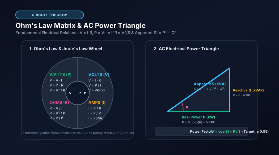
Concurrently, Joule's First Law (published by James Prescott Joule in 1841) describes the thermodynamic transformation of electrical potential energy into thermal kinetic energy (Joule heating). As charge carriers transfer kinetic momentum to the crystal lattice via inelastic phononic scattering, the irreversible rate of energy dissipation is given by P = dW/dt = V × I = I²R = V²/R. This 12-form algebraic wheel forms the bedrock of all electrical circuit analysis.
2. Topological Circuit Theorems: Series, Parallel, and Delta-Wye Networks
Real-world power distribution grids, instrumentation amplifiers, and passive attenuator pads involve complex interconnected networks that can be systematically reduced using Kirchhoff's fundamental conservation laws:
- Kirchhoff's Current Law (KCL): Rooted in the conservation of electric charge, the algebraic sum of currents entering any electrical node must equal zero (Σ I_in = Σ I_out). In parallel resistor topologies, this dictates that reciprocal resistances (conductances G = 1/R) add linearly.
- Kirchhoff's Voltage Law (KVL): Rooted in the conservative nature of static electrostatic fields (∮ E • dl = 0), the directed sum of potential differences around any closed circuit loop equals zero. In series resistor topologies, voltages divide in direct proportion to resistance.
- Kennelly's Delta-to-Wye (Δ-Y) Transformation: Devised by Arthur Edwin Kennelly in 1899, this three-terminal network equivalence theorem transforms bridge networks that are neither purely series nor purely parallel into simplified star configurations, resolving complex Wheatstone bridge imbalances and 3-phase power transformer loads without resorting to 3×3 matrix nodal inversion.
3. The Loaded Voltage Divider & Thevenin's Loading Effect
A common trap in novice electronic engineering is assuming that an ideal voltage divider maintains its nominal output ratio when connected to a downstream circuit. Consider two divider resistors R₁ and R₂ powered by V_in. While the unloaded voltage is V_out = V_in × [R₂ / (R₁ + R₂)], connecting any physical load resistance R_L across the output creates an effective bottom impedance of R₂_eff = (R₂ × R_L) / (R₂ + R_L).
Because R₂_eff is strictly less than R₂, the actual output voltage sags below its design value. According to Thevenin's Theorem, any linear two-terminal network can be modeled as an ideal voltage source V_th in series with an output impedance R_th = R₁ ∥ R₂. To prevent loading error from exceeding 1%, standard electronic design practice dictates that the load resistance must satisfy R_L ≥ 100 × R_th. When high impedance drive is unfeasible due to excessive quiescent battery drain, an active operational amplifier unity-gain buffer must be placed between the divider and the load.
4. Solid-State LED Ballast Biasing and Thermal Runaway Prevention
Light-Emitting Diodes (LEDs) are non-linear minority-carrier injection semiconductor devices exhibiting an exponential Shockley diode I-V characteristic:
Because the diode forward voltage drop V_f possesses a negative temperature coefficient (typically -1.5 to -2.5 mV/°C for gallium-nitride and indium-gallium-aluminum-phosphide junctions), powering an LED directly from a stiff voltage source without a ballast impedance leads to catastrophic thermal runaway: heating decreases V_f, which exponentially accelerates current draw, driving further self-heating until the semiconductor bond wire or junction melts.
A passive series ballast resistor converts the voltage source into an approximate current regulator, establishing a negative feedback loop: an increase in current induces a larger voltage drop across the resistor, reducing the voltage across the LED. For robust commercial reliability, engineers must apply a 50% derating factor to the resistor's continuous wattage rating (P_rating ≥ 2 × P_dissipated) to keep ambient surface temperatures below flammable thresholds.
Frequently Asked Questions (Institutional FAQ)
Why can't I connect multiple LEDs directly in parallel with a single shared resistor?▼
Even LEDs from the same semiconductor manufacturing wafer batch have minute variations in forward voltage drop (ΔV_f ≈ 20-50 mV). Because the I-V curve is exponential, the LED with the lowest V_f will hog current (current hogging), running significantly hotter than its peers. As it heats up, its V_f drops even further, causing it to burn out first, followed in rapid succession by the remaining over-driven LEDs. Always provide each parallel branch with its own dedicated ballast resistor.
What are E-series standard resistor values (E12, E24, E96)?▼
Defined by International Electrotechnical Commission standard IEC 60063, E-series numbers represent logarithmic preferred values that ensure adjacent resistor tolerances overlap without unnecessary production gaps. E12 offers 12 steps per decade (±10% tolerance), E24 offers 24 steps per decade (±5% tolerance), and E96 offers 96 steps per decade (±1% high-precision metal film resistors).
How does resistor temperature coefficient (TCR) affect precision dividers?▼
Resistors experience resistance changes with temperature: R(T) = R₀ × [1 + α(T - T₀)], where α is the Temperature Coefficient of Resistance (expressed in ppm/°C). Standard thick-film resistors have TCRs of ±100 to ±200 ppm/°C. In precision voltage dividers for analog-to-digital converters (ADCs), mismatched thermal coefficients between R1 and R2 can cause drift. Using matched thin-film resistor arrays with TCR tracking within 2-5 ppm/°C prevents thermal measurement drift.