
1. Foundations of Managerial Accounting & Profit Architecture
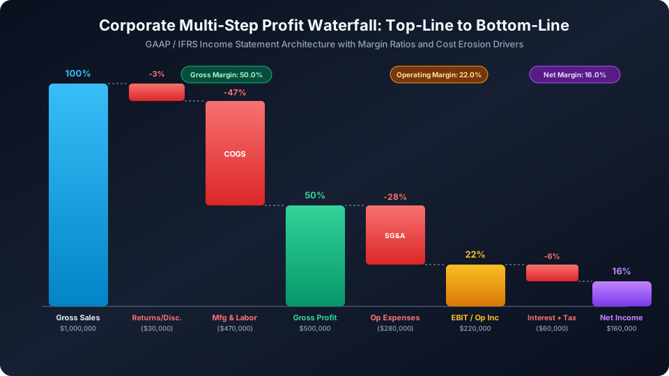
Corporate profitability analysis is the cornerstone of managerial accounting, financial valuation, and corporate treasury management. Under international standards (both US GAAP ASC 330 and IFRS IAS 2), profitability is not measured as an isolated static figure; rather, it is dissected across a multi-tier financial waterfall that distinguishes between prime product costs, period operational expenses, and capital structure financing charges.
At the top of the waterfall, Gross Profit gauges the fundamental viability of an organization’s production or service delivery model. It compares net sales revenue directly against the Cost of Goods Sold (COGS). A company that cannot sustain healthy gross profit margins cannot survive long-term, regardless of how lean its corporate headquarters or administrative overhead may be. Conversely, Net Profit reflects the ultimate bottom line available to common shareholders or reinvestment, incorporating all corporate operating expenditures (SG&A, research and development, marketing), asset depreciation and amortization, debt service interest, and statutory corporate income taxes.
1.1 Gross Profit Margin vs. Markup: The Fundamental Pricing Confusion
One of the most persistent errors encountered in small business management and corporate pricing strategy is the conflation of Margin and Markup. While both metrics quantify the difference between product cost and selling price, they utilize completely different mathematical denominators:
- Gross Profit Margin (%) is calculated relative to Selling Price (Revenue):
Gross Margin = (Selling Price - COGS) ÷ Selling Price - Markup (%) is calculated relative to Cost of Goods Sold:
Markup = (Selling Price - COGS) ÷ COGS
For example, if an enterprise manufactures a specialized electronic component for $50 and sells it for $100, the absolute gross profit is $50. The markup on cost is 100% ($50 ÷ $50), but the gross profit margin is 50% ($50 ÷ $100). Miscalculating this distinction frequently leads businesses to price goods below their operating break-even threshold, resulting in unanticipated operational cash drain.
2. Inventory Cost Flow & Cost of Goods Sold (COGS) Engineering
For manufacturing and retail enterprises, inventory constitutes one of the largest working capital assets on the balance sheet. Cost of Goods Sold is the expense recognized when inventory is transferred to buyers. The universal periodic inventory identity is defined as:
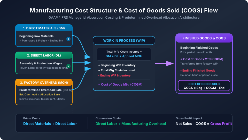
In a full absorption manufacturing environment, this formula expands into a multi-phase production lifecycle:
- Raw Materials Incurred: Beginning Raw Materials + Purchases of Raw Materials - Ending Raw Materials = Direct Materials Consumed in Production.
- Work In Process (WIP) Conversion: Direct Materials Consumed + Direct Manufacturing Labor + Applied Factory Overhead = Total Manufacturing Costs Incurred during the period.
- Cost of Goods Manufactured (COGM): Beginning WIP + Total Manufacturing Costs Incurred - Ending WIP = Cost of Goods Manufactured (the cost of units finished and moved to the warehouse).
- Cost of Goods Sold (COGS): Beginning Finished Goods Inventory + COGM - Ending Finished Goods Inventory = Final Cost of Goods Sold recognized on the income statement.
2.1 Predetermined Overhead Allocation Rates (POHR)
Indirect factory expenses—such as supervisory wages, plant utility power, factory machinery depreciation, lubricants, and security—cannot be traceably assigned to a single finished product. Consequently, cost accountants establish a Predetermined Overhead Rate (POHR) prior to the start of the fiscal year:
Common cost allocation drivers include:
- Direct Labor Hours (DLH): Ideal for labor-intensive assembly processes where human labor duration directly correlates with factory utility and supervisory consumption.
- Machine Hours (MH): The standard in automated robotics, semiconductor fabrication, and CNC machining, where machine run-time drives power consumption and equipment wear.
- Direct Labor Cost ($): Utilized when wage differentials are stable and payroll tracking serves as an automated surrogate for manufacturing complexity.
3. Cost-Volume-Profit (CVP) Dynamics: Target Profit & Margin of Safety
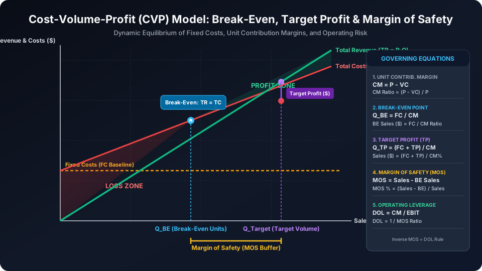
Cost-Volume-Profit (CVP) analysis examines the interplay between sales volume, product pricing, variable unit costs, and total fixed expenses. CVP modeling relies on the foundational concept of the Contribution Margin (CM):
Contribution Margin Ratio (CM%) = Unit CM ÷ Selling Price = Total CM ÷ Total Revenue
The contribution margin represents the incremental cash flow generated by each unit sold that contributes toward covering fixed operational costs. Once cumulative contribution margin equals total fixed costs, the enterprise achieves its Break-Even Point (BEP).
3.1 Target Profit Analysis: Pre-Tax vs. After-Tax Formulations
Corporate executives routinely require sales targets designed to hit specific earnings hurdles. When management establishes a target profit goal ($TP$), the required unit sales volume ($Q_{target}$) is derived by expanding the break-even equation:
If the corporate target is defined on an after-tax net income basis ($NI_{target}$), the after-tax figure must first be grossed up by the corporate effective tax rate ($t$):
3.2 The Margin of Safety (MOS) Cushion
The Margin of Safety (MOS) quantifies the degree to which sales can drop before the enterprise encounters operating losses. It is expressed in three distinct forms:
- MOS in Dollars: Current Actual/Budgeted Revenue - Break-Even Revenue.
- MOS in Units: Current Unit Sales Volume - Break-Even Unit Volume.
- MOS Ratio (%): (Margin of Safety in Dollars ÷ Current Sales Revenue) × 100.
A high Margin of Safety indicates robust financial insulation against macroeconomic recessions, price wars, or raw material cost spikes. In contrast, an MOS below 15% signals acute vulnerability to minor demand shocks.
4. The Theory of Enterprise Leverage: DOL, DFL & DCL
In corporate finance and capital structure optimization, Leverage refers to the use of fixed costs to magnify returns to capital providers. Leverage operates as a double-edged sword: in periods of sales growth, it propels earnings upward at an accelerated velocity; during downturns, it triggers catastrophic collapses in operating cash flows and solvency.
4.1 Degree of Operating Leverage (DOL)
The Degree of Operating Leverage (DOL) measures the elasticity or sensitivity of a company’s operating income (EBIT) relative to changes in top-line sales volume. It arises entirely from the presence of fixed operating costs (such as factory rent, automated plant depreciation, executive salaries, and software licenses) in the cost structure:
Crucially, there is an exact reciprocal mathematical relationship between DOL and the Margin of Safety:
When a business operates near its break-even point, its Margin of Safety approaches zero, driving its DOL toward infinity. At this threshold, a mere 1% uptick in sales can trigger a 50% surge in EBIT.
4.2 Degree of Financial Leverage (DFL)
While DOL stems from production and operating decisions, the Degree of Financial Leverage (DFL) originates from the firm’s capital structure decisions—specifically, the issuance of fixed-charge debt (bank loans, bonds) or preferred stock. DFL quantifies the percentage change in Earnings Per Share (EPS) or EBT resulting from a 1% change in EBIT:
If a firm has zero debt and zero preferred equity, its DFL is exactly 1.0 (no financial amplification). As debt obligations expand, fixed interest deductions eat into EBIT, escalating financial risk and magnifying equity return volatility.
4.3 Degree of Combined Leverage (DCL): Total Risk Magnification
The total sensitivity of a company's bottom-line net income and EPS to fluctuations in top-line sales volume is captured by the Degree of Combined Leverage (DCL). It is the multiplicative product of operating and financial leverage:
The Enterprise Leverage Trade-Off Matrix:
| Leverage Profile | Operating Cost (DOL) | Debt Financing (DFL) | Typical Industry Archetype | Risk / Return Trade-Off |
|---|---|---|---|---|
| Conservative | Low Fixed Costs | Zero / Low Debt | Professional Services, Wholesalers | Low risk; highly resilient in downturns, limited profit explosion in booms. |
| Capital-Intensive | High Fixed Costs | Conservative Debt | SaaS, Semiconductor Foundries, Cloud Infrastructure | Massive margin expansion once past break-even; low bankruptcy threat from debt. |
| Financially Leveraged | Low Fixed Costs | High Debt Load | Real Estate Syndicates, Private Equity LBOs | Stable operating margins support debt service; vulnerable to benchmark rate spikes. |
| High Risk Hazard | High Fixed Costs | Heavy Debt Load | Legacy Airlines, Steel Mills, Commercial Real Estate Developers | Extreme default risk. A 10% revenue drop frequently wipes out 100% of equity earnings. |
5. Practical Enterprise Implementation & CFO Decision Checklist
Corporate treasury officers and financial planning & analysis (FP&A) leaders leverage these ten tools continuously throughout the annual budget cycle:
- Quarterly Gross Margin Audits: Track direct material price variance and labor efficiency variances against standard costs to prevent margin leakage before quarterly reports.
- Overhead Under/Over-Absorption Review: At fiscal year-end, reconcile applied overhead against actual factory expenditures. If actual overhead exceeds applied overhead, debit COGS to account for under-applied variance.
- Sensitivity Stress-Testing: Apply the Combined Leverage multiplier (DCL) to downside economic scenarios (-10%, -20% sales demand) to verify whether projected operating income maintains minimum Debt Service Coverage Ratios (DSCR > 1.35×) stipulated in bank covenants.
- Capital Expenditure (CapEx) Trade-Off Evaluation: Before automating a manufacturing line (converting variable labor costs into fixed machinery depreciation), evaluate whether the resulting spike in DOL leaves adequate Margin of Safety for volatile market conditions.