Matrix & Vector Grid
System Solution & Spectrum
Computed Solution
λ₁ = 3.6180, λ₂ = 1.3820
Expression: Eigensystem of 2×2 Principal Minor [[2, 1], [1, 3]]
Analytical Derivation & Invariants
1Characteristic Polynomial: λ² - Tr(A)λ + det(A) = λ² - 5.000λ + 5.000 = 0
2Discriminant Δ = Tr(A)² - 4·det(A) = 5.0000 (Real roots)
3Eigenvalue λ₁: 3.6180 with Eigenvector v₁ ≈ [0.618, 1.000]ᵀ
4Eigenvalue λ₂: 1.3820 with Eigenvector v₂ ≈ [-1.618, 1.000]ᵀ
5Eigenvalue Sum Check: λ₁ + λ₂ = 5.0000 = Tr(A) = 5.0000
6Eigenvalue Product Check: λ₁ · λ₂ = 5.0000 = det(A) = 5.0000
Visual Linear Systems Architecture
Matrix transformations, span, Gaussian RREF, eigensystem spectrum, SVD geometry, and PCA dimensionality reduction.
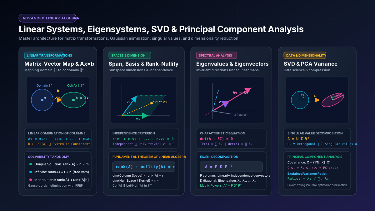
1. Linear Transformations and Matrix-Vector Operator Mechanics
A linear transformation is a mathematical mapping T: ℝⁿ → ℝᵐ preserving vector addition and scalar multiplication: T(u + v) = T(u) + T(v) and T(cu) = cT(u). By the foundational representation theorem of linear algebra, every linear transformation between finite-dimensional spaces can be represented uniquely by an m × n matrix A, such that T(x) = Ax.
The product \(Ax\) has two complementary interpretations:
- Row View (Dot Products): The \(i\)-th component of the output vector \(b\) is the dot product of row \(i\) of \(A\) with input vector \(x\).
- Column View (Linear Combination): The output vector \(b\) is a weighted linear combination of the columns of \(A\): \(Ax = x_1 a_1 + x_2 a_2 + \dots + x_n a_n\).
2. Solving Linear Systems: The Geometry of Ax = b and Gaussian Elimination
The fundamental problem of linear algebra is solving the linear system \(Ax = b\). Based on the Rouché-Capelli Theorem, the augmented matrix \([A \mid b]\) determines the exact nature of the solution space:
Unique Solution
rank(A) = rank[A | b] = n. The determinant det(A) ≠ 0; the matrix is invertible, and x = A⁻¹b.
Infinite Solutions
rank(A) = rank[A | b] = r < n. There are n - r free variables, yielding a parametric affine subspace.
Inconsistent (No Solution)
rank(A) < rank[A | b]. The target vector b does not lie in the column space Col(A).
3. The Fundamental Theorem of Linear Algebra & Rank-Nullity
For any linear transformation represented by an m × n matrix A, the domain ℝⁿ and codomain ℝᵐ split into Gilbert Strang's four fundamental subspaces:
- Column Space Col(A): Subspace of ℝᵐ spanned by the columns; dim Col(A) = r (the rank).
- Null Space Null(A): Solution space to Ax = 0 in ℝⁿ; dim Null(A) = n - r (the nullity).
- Row Space Row(A): Subspace of ℝⁿ spanned by the rows; dim Row(A) = r.
- Left Null Space Null(Aᵀ): Solutions to Aᵀ y = 0 in ℝᵐ; dim Null(Aᵀ) = m - r.
The celebrated Rank-Nullity Theorem formalizes this conservation of dimension:
rank(A) + nullity(A) = n (number of columns)
4. Spectral Analysis: Eigenvalues, Eigenvectors, and Diagonalization
When a matrix A acts on most vectors, it changes both their length and direction. However, certain special non-zero vectors v maintain their directional axis, undergoing pure scaling by a scalar factor λ:
A v = λ v ⟺ (A - λ I) v = 0
Non-trivial solutions exist if and only if the characteristic polynomial vanishes: det(A - λ I) = 0. If A possesses n linearly independent eigenvectors, it can be diagonalized as A = P D P⁻¹, where D is a diagonal matrix of eigenvalues. Diagonalization allows computing high matrix powers effortlessly: Aᵏ = P Dᵏ P⁻¹.
5. Singular Value Decomposition (SVD): The Pinnacle of Matrix Factorization
While eigendecomposition requires square, diagonalizable matrices, the Singular Value Decomposition (SVD) exists for any real or complex m × n matrix A:
A = U Σ Vᵀ
Here, U is an m × m orthogonal matrix of left singular vectors (eigenvectors of A Aᵀ), V is an n × n orthogonal matrix of right singular vectors (eigenvectors of Aᵀ A), and Σ is an m × n diagonal matrix containing non-negative singular values σ₁ ≥ σ₂ ≥ ... ≥ σ_r > 0.
Geometrically, SVD reveals that every linear transformation can be decomposed into: (1) an orthogonal rotation Vᵀ, (2) coordinate stretching along principal axes by σ_i, and (3) a second orthogonal rotation U. By the Eckart-Young-Mirsky Theorem, truncating the SVD to the top k singular values yields the provably optimal rank-k approximation of matrix A under Frobenius and spectral norms.
6. Principal Component Analysis (PCA) and Dimensionality Reduction
In modern machine learning and high-dimensional data science, Principal Component Analysis (PCA) is the unsupervised technique for discovering the orthogonal directions of maximum variance. For a mean-centered data matrix X̃, the sample covariance matrix is:
C = (1 / (N - 1)) X̃ᵀ X̃
The eigenvectors of C define the principal component directions w₁, w₂, ..., w_p, and the corresponding eigenvalues λ_i quantify the variance explained along each axis. The explained variance ratio λ_i / ∑ λ_k provides the quantitative justification for compressing hundreds of raw features into a compact, uncorrelated feature embedding with minimal information loss.