Gauss-Markov Ordinary Least Squares Engine
Linear Regression, Pearson & Covariance Suite
Derive Ordinary Least Squares (OLS) slope coefficients, R² goodness-of-fit, Pearson & Spearman rank correlations, 2×2 covariance matrices, and calibrated value extrapolations.
Bivariate Dataset Input (X and Y Pairs)
Enter matching sequences of values separated by commas, spaces, or tabs. Both variables must have equal length.
Visual Guide 1
OLS Linear Regression & Scatterplot Geometry
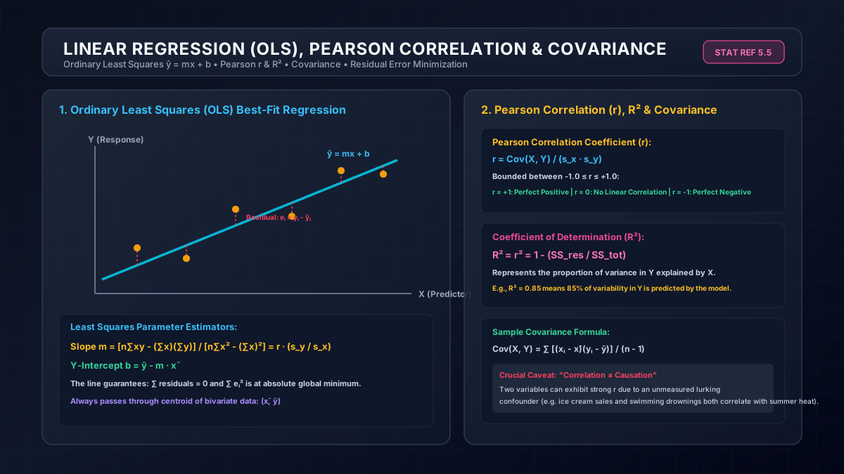
Figure 1.0: Vector decomposition of squared vertical residuals, slope m, intercept b, and regression plane.
Visual Guide 2
Descriptive Statistics & Marginal Dispersion

Figure 2.0: Structural relation between univariate marginal spreads and joint bivariate covariances.
Bivariate Stochastic Modeling: Ordinary Least Squares, Pearson Correlation & Covariance Matrices
Bivariate statistics studies the empirical relationship and joint variability between two quantitative random variables X and Y. From financial Capital Asset Pricing Models (CAPM Beta) and econometric trend forecasting to machine learning linear predictors, Ordinary Least Squares (OLS) regression and correlation analysis remain foundational workhorses of quantitative analysis.
1. The Gauss-Markov Theorem & Ordinary Least Squares (OLS)
The Gauss-Markov theorem states that under five fundamental classical assumptions, the Ordinary Least Squares estimator is the Best Linear Unbiased Estimator (BLUE)—meaning it achieves minimum variance among all possible unbiased linear estimators:
- Linearity in Parameters: The true data-generating process is linear: Y_i = β₀ + β₁ X_i + ε_i.
- Strict Exogeneity: The expected value of errors given X is zero: E[ε_i | X_i] = 0.
- Homoscedasticity: Constant error variance across all values of X: Var(ε_i | X_i) = σ².
- No Autocorrelation: Residual errors are uncorrelated between different observations: Cov(ε_i, ε_j) = 0 for i ≠ j.
- Non-Collinearity: The independent variable X possesses non-zero variance.
2. Mathematical Derivation of OLS Slope and Intercept
The objective of OLS is to find parameters m and b that minimize the sum of squared vertical residuals:
S(m, b) = Σ [ y_i - (m · x_i + b) ]²
Taking partial derivatives with respect to m and b and setting them equal to zero produces the normal equations, yielding:
m = Σ (x_i - x̄)(y_i - ȳ) / Σ (x_i - x̄)² = Cov(X, Y) / Var(X) = r · (s_y / s_x)
b = ȳ - m · x̄
This demonstrates that the regression line always passes directly through the centroid of the data: (x̄, ȳ).
3. Coefficient of Determination (R²) and Goodness-of-Fit
Total variation in the dependent variable (SST) decomposes into explained sum of squares (SSR) and residual error (SSE):
Σ (y_i - ȳ)² = Σ (ŷ_i - ȳ)² + Σ (y_i - ŷ_i)² ⟺ SST = SSR + SSE
The Coefficient of Determination R² represents the fraction of total variance in Y explained by the linear model:
R² = 1 - SSE / SST = SSR / SST = r²
In simple bivariate regression, R² is exactly the square of the Pearson correlation coefficient r. An R² of 0.85 indicates that 85% of variation in Y is linearly attributable to X, with the remaining 15% relegated to unexplained random disturbance.
4. Pearson r vs. Spearman Rank ρ
Pearson Correlation (r)
Measures the strength and direction of purely linear associations between continuous, normally distributed variables:
r = Σ (x - x̄)(y - ȳ) / √[ Σ (x - x̄)² · Σ (y - ȳ)² ]
Highly sensitive to severe outliers, which can falsely inflate or collapse r.
Spearman Rank (ρ)
A non-parametric metric that measures monotonic relationships (whether Y always increases when X increases, regardless of curvature):
ρ = 1 - [6 Σ d_i²] / [n(n² - 1)]
Robust to non-linear exponential curves and extreme outliers because it operates on ranks rather than raw magnitudes.