Enter Dataset
Separate numbers with commas, spaces, or line breaks.
Preset Datasets:
Please enter valid numerical data in the box on the left.
Institutional Statistics ReferenceData Analysis & Empirical Methods
The Comprehensive Handbook of Descriptive Statistics, Dispersion, and Data Distributions
Descriptive statistics distill complex raw datasets into concise, actionable mathematical summaries. From central tendency and Bessel's variance correction to Tukey's boxplots and higher-order moments, this reference provides the rigorous mathematical framework underlying scientific data exploration.

Figure 1: Central Tendency, Five-Number Summary, Tukey Outlier Fences, and Distribution Asymmetry.
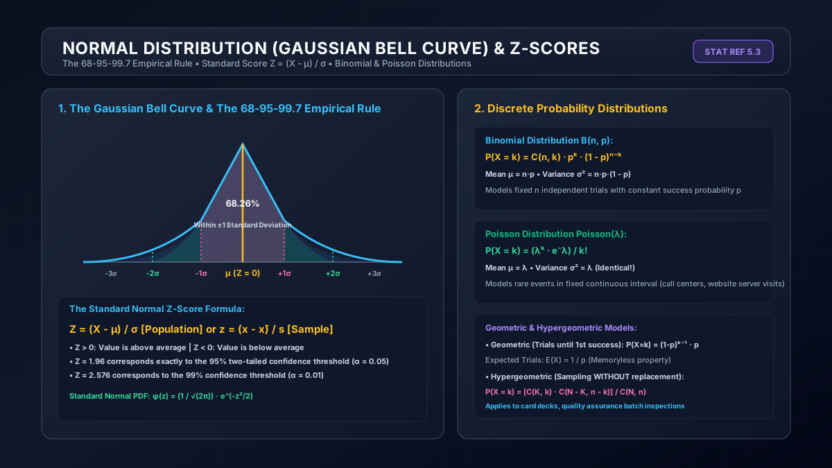
Figure 2: The Empirical Rule (68-95-99.7%) and Standard Normal Z-Score Transformation.
1. Measures of Central Tendency: Mean, Median, and Mode
Central tendency quantifies the center point or typical value of a probability distribution or dataset:
- Arithmetic Mean (x̄): The sum of all values divided by count n: x̄ = (∑ xᵢ) / n. The mean minimizes the sum of squared deviations ∑ (xᵢ - c)², but is sensitive to extreme outliers.
- Median (M): The 50th percentile dividing ordered data into two equal halves. The median minimizes the sum of absolute deviations ∑ |xᵢ - c|, making it robust against heavily skewed data (such as national income or housing prices).
- Mode: The most frequently occurring score in the dataset. Unimodal distributions have one mode; bimodal distributions exhibit two peaks.
2. Dispersion & Why Bessel's Correction (n - 1) Is Essential
When computing the variance of an entire population of size N, we divide by N:
σ² = ∑ (xᵢ - μ)² / N
However, when estimating variance from a sample of size n, using the sample mean x̄ instead of true population mean μ systematically underestimates the true variance because sample deviations are calculated relative to their own center. Friedrich Bessel proved that dividing by (n - 1) yields an unbiased estimator whose expected value equals the true population variance:
s² = ∑ (xᵢ - x̄)² / (n - 1) ⟹ E[s²] = σ²
3. Five-Number Summary, IQR, and Tukey's Outlier Rule
Introduced by John Tukey in 1977, the box-and-whisker plot summarizes a distribution using five key values: Minimum, First Quartile (Q₁), Median (Q₂), Third Quartile (Q₃), and Maximum.
The Interquartile Range (IQR = Q₃ - Q₁) encompasses the middle 50% of the data. Data points falling beyond the standard Tukey fences are flagged as statistical outliers:
Lower Outlier Fence = Q₁ - 1.5 × IQR
Upper Outlier Fence = Q₃ + 1.5 × IQR