Math Calculator
Probability & Statistics
Parametric Stochastic Density Engine
Normal, Binomial, Poisson & Z-Score Suite
Compute cumulative probabilities, standardized Z-scores, Gaussian densities, discrete Bernoulli trials, Poisson arrival rates, and finite Hypergeometric sampling with zero approximation drift.
Normal Distribution (Mean μ, Std Dev σ) & Z-Score
Calculate cumulative area under the Gaussian bell curve or determine the raw threshold X given a standardized Z score.
Standard normal uses 0
Standard normal uses 1
Visual Guide 1
Gaussian Normal & Standard Z-Distribution Curve
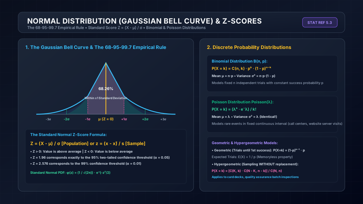
Figure 1.0: Vector decomposition of the 68-95-99.7 empirical rule, inflection points, and tail probability areas.
Visual Guide 2
Discrete Sampling & Combinatorial Tree Architectures

Figure 2.0: Mapping Bernoulli trials, replacement rules, and hypergeometric combinatorial partitions.
Parametric Probability Density & Cumulative Distribution Functions
Probability distributions are formal mathematical functions that assign probabilities to different outcomes of a random phenomenon. They represent the foundational apparatus for inferential statistics, quality engineering, econometric forecasting, and machine learning architectures.
1. The Gaussian Normal Distribution (μ, σ²)
The normal (or Gaussian) distribution is ubiquitous because of the Central Limit Theorem (CLT), which asserts that the normalized sum of independent and identically distributed random variables converges toward a normal distribution as sample size n grows large, regardless of the underlying distribution’s shape.
f(x | μ, σ²) = [1 / (σ √(2π))] · exp(-(x - μ)² / (2σ²))
Key analytical properties of the Gaussian distribution include:
- Symmetry: Perfect reflectional symmetry around the mean μ, meaning Mean = Median = Mode. Skewness is identically zero.
- Inflection Points: The concave downward bell curve transitions to concave upward at exactly x = μ ± σ.
- Empirical Rule (68–95–99.7): Approximately 68.27% of observations lie within ±1σ, 95.45% within ±2σ, and 99.73% within ±3σ.
2. Standardized Z-Scores and Standard Normal Table
To compare observations across disparate distributions without numerically integrating the non-elementary Gaussian integral for each unique pair of (μ, σ), variables are transformed to standard normal space N(0, 1) via the Z-transformation:
Z = (X - μ) / σ ⟺ X = μ + Z·σ
The standard normal cumulative distribution function Φ(z) satisfies Φ(z) = 0.5 · [1 + erf(z / √2)]. Standard critical Z-thresholds include Z = 1.645 for a 90% two-tailed confidence level (α = 0.10), Z = 1.96 for a 95% confidence level (α = 0.05), and Z = 2.576 for a 99% confidence level (α = 0.01).
3. The Binomial Distribution B(n, p)
The binomial distribution models the discrete count of successes in a sequence of n independent experiments (Bernoulli trials), each having a constant probability of success p:
P(X = k) = nCr(n, k) · p^k · (1 - p)^(n - k) for k ∈ [0, 1, ..., n]
The mean is E[X] = n × p, and the variance is Var(X) = n × p × (1 - p). When n is sufficiently large and p is not near 0 or 1 (specifically np ≥ 5 and n(1-p) ≥ 5), the Binomial distribution can be reliably approximated by the normal distribution N(np, np(1-p)) with a continuity correction factor of ±0.5.
4. The Poisson Distribution (λ)
Developed by Siméon Denis Poisson, this distribution expresses the probability of a given number of events occurring in a fixed interval of time or space, assuming events arrive independently at a constant average rate λ:
P(X = k) = (λ^k · e^-λ) / k! for k ∈ [0, 1, 2, ...]
A distinctive property of the Poisson distribution is equidispersion, where the theoretical mean and variance are identical: E[X] = Var(X) = λ. When sample variance exceeds the mean in empirical counting datasets, the condition is termed overdispersion, often requiring Negative Binomial modeling.
5. Geometric & Hypergeometric Sampling Models
Geometric Distribution
Models the number of independent Bernoulli trials required to achieve the very first success:
P(X = k) = (1 - p)^(k - 1) · p
It possesses the unique memoryless property among discrete distributions: P(X > s + t | X > s) = P(X > t).
Hypergeometric Distribution
Evaluates sampling without replacement from a finite population of size N containing K successes:
P(X = k) = [nCr(K, k) · nCr(N - K, n - k)] / nCr(N, n)
As population N grows large relative to sample size n (n/N < 0.05), hypergeometric probabilities converge directly to binomial probabilities.
Frequently Asked Questions (Academic & Industrial FAQ)
About Z-Score Calculator
Parametric probability distributions suite. Calculate Gaussian normal curves, Z-scores, Binomial B(n,p), Poisson arrival rates, Geometric trials, and finite Hypergeometric sampling with zero approximation drift.
Why this page helps
- Zero approximation drift for critical alpha levels (90%, 95%, 99%) and quality control six-sigma bounds
- Standardizes disparate datasets for cross-comparative grading, psychometrics, and financial risk
- Accelerates statistical modelling for industrial reliability and inventory queueing
How to use it well
- Select your distribution category: Gaussian Normal & Z-Score, Discrete Binomial / Poisson, or Geometric / Hypergeometric.
- Input distribution parameters (mean μ, standard deviation σ, number of trials n, probability p, or rate λ).
- Choose between calculating cumulative probability P(X ≤ x), exact point probability P(X = k), or solving raw value X from a target Z-score.
- Review probability density, cumulative CDF area, expected value E[X], and distribution variance.