Math Calculator
Probability & Statistics
Neyman-Pearson & Fisherian Testing Engine
Hypothesis Testing, t-Test, Chi-Square & ANOVA Suite
Execute 1-sample & 2-sample Welch t-tests, exact P-values, Chi-Square cross-tabulations, One-Way ANOVA F-tests, two-sided confidence intervals, and statistical power sample size sizing.
Student’s t-Distribution Inference
One-sample mean comparison or two-sample Welch’s t-test with unequal variance support.
Sample Parameters
Visual Guide 1
Hypothesis Testing & Significance Decision Architecture

Figure 1.0: Null vs. alternative distributions, Type I (α) and Type II (β) error tradeoffs, and P-value mapping.
Visual Guide 2
Gaussian Normal Standard & Critical Cutoff Geometry
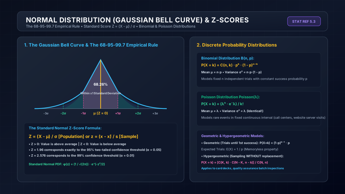
Figure 2.0: The standard normal Z-transformation geometry, two-tailed tail regions, and 95% critical acceptance regions.
Inferential Statistical Decision Theory: t-Tests, P-Values, Chi-Square & Power Analysis
Inferential statistics enables scientists, biomedical researchers, quantitative financial traders, and engineers to draw rigorous conclusions regarding unobservable population parameters from finite, stochastic sample observations. Rather than stating qualitative opinions, hypothesis testing formalizes decision boundaries under probabilistic uncertainty.
1. Neyman-Pearson Decision Framework vs. Fisherian Significance
Modern inferential testing synthesizes two distinct historical methodologies:
- Ronald Fisher’s P-Value Approach: Focuses on a single hypothesis—the Null Hypothesis (H₀). The p-value represents the conditional probability P(D ≥ d_obs | H₀) of observing data at least as extreme as the current sample, assuming H₀ is true. It serves as an index of evidence against the null, with no explicit alternative hypothesis specified.
- Jerzy Neyman & Egon Pearson’s Decision Theory: Establishes two competing statistical models: H₀ versus an Alternative Hypothesis (Ha). Before collecting data, the experimenter selects an acceptable false-positive risk α (Type I error) and designs the trial to minimize false negatives β (Type II error), maximizing Statistical Power (1 - β).
2. Student’s t-Distribution & Degrees of Freedom
When population variance σ² is unknown and must be estimated via sample variance s², the standardized variable follows William Sealy Gosset’s Student’s t-distribution rather than a normal distribution:
t = (x̄ - μ₀) / (s / √n) ~ t(df = n - 1)
The t-distribution has heavier tails than the normal curve to compensate for the additional uncertainty of estimating σ. As sample size n grows large, the degrees of freedom df grow, and the t-distribution converges asymptotically to the standard Gaussian normal distribution N(0, 1).
For comparing two independent groups without assuming equal variances, Welch’s t-test must be used instead of Student’s pooled t-test. The Welch-Satterthwaite approximation computes degrees of freedom as:
df_Welch = [(s₁²/n₁ + s₂²/n₂)²] / [ (s₁²/n₁)² / (n₁ - 1) + (s₂²/n₂)² / (n₂ - 1) ]
3. Chi-Square (χ²) Test of Independence
Used to evaluate associations between categorical variables arranged in an r × c contingency table. Under the null hypothesis of independence, expected frequencies are computed as E_ij = (R_i × C_j) / N. The Pearson Chi-Square test statistic is:
χ² = Σ Σ (O_ij - E_ij)² / E_ij with df = (r - 1)(c - 1)
Cochran’s Criteria: The asymptotic Chi-Square approximation is mathematically valid only when no cell has an expected frequency less than 1, and no more than 20% of cells have expected counts less than 5. If violated, Fisher’s Exact Test must be employed.
4. One-Way Analysis of Variance (ANOVA)
When comparing means across k ≥ 3 groups, conducting pairwise t-tests causes catastrophic inflation of the family-wise error rate (α_family = 1 - (1 - α)^m). ANOVA resolves this by partitioning total sum of squares (SST) into between-group variance (SSB) and within-group error variance (SSW):
F = MSB / MSW = [SSB / (k - 1)] / [SSW / (N - k)]
If between-group variation significantly exceeds within-group random error (F > F_critical), the null hypothesis that all group means are identical is rejected. Post-hoc testing (Tukey’s HSD or Bonferroni correction) is subsequently conducted to locate specific pair differences.
5. Statistical Power & Sample Size Determination
Underpowered studies fail to detect true clinical or scientific effects, wasting capital and patient trials. Sample size sizing via Cochran’s formula establishes minimum required participants:
n₀ = [Z² · p(1 - p)] / E² ⟹ n_adj = n₀ / [1 + (n₀ - 1) / N]
Where Z corresponds to desired confidence (1.96 for 95%), p is the estimated proportion (0.50 provides maximum variance and the most conservative sample estimate), and E is allowable margin of error. If sampling from a known finite population N, the Finite Population Correction (FPC) prevents excessive oversampling.
Frequently Asked Questions (Academic & Clinical FAQ)
About T-Test Calculator
Institutional hypothesis testing and inferential statistics suite. Execute 1-sample & 2-sample Welch t-tests, exact P-values, Chi-Square contingency tables, One-Way ANOVA F-tests, confidence intervals, and survey sample size sizing.
Why this page helps
- Prevents false-positive conclusions using Welch-Satterthwaite unequal variance adjustments
- Optimizes clinical trial and survey research budgets by calculating exact minimum statistical power sample sizes
- Delivers complete academic ANOVA and Chi-Square summary tables for research publications
How to use it well
- Select your inferential method: Student's t-Test & P-Value, Chi-Square & ANOVA, or Confidence Interval & Sample Sizing.
- Input your sample statistics (sample mean, standard deviation, sample size, or categorical frequencies).
- Set your confidence level (e.g. 95%, 99%) and significance threshold α (0.05, 0.01).
- Evaluate test statistics (t, F, χ²), exact p-values, Cohen's d effect sizes, and reject/fail-to-reject decision outcomes.