Applied Energy, Power Engineering & Battery Lifecycle Optimization
A comprehensive treatise on electrochemical cell storage, multi-stage CC/CV charging, grid tariffs, IoT energy harvesting, and wave radiation geometry.
1. Electrochemical Cell Storage & Peukert's Law Derating
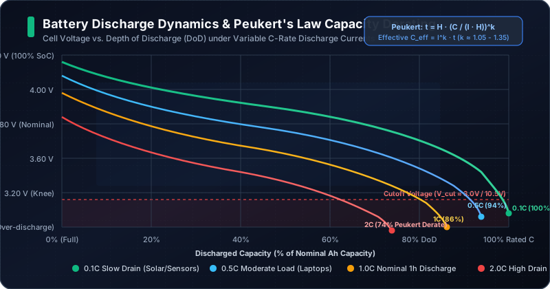
Secondary (rechargeable) battery cells do not behave like ideal static reservoirs of electrical charge. When current is drawn from an electrochemical cell, active ionic species (such as lithium ions in Li-ion chemistry or lead sulfate ions in lead-acid chemistry) must physically migrate through electrolyte solutions and solid electrode porous matrices. At low discharge rates (such as a 20-hour rate, or 0.05C), ions have sufficient time to diffuse evenly throughout the active cathode material, allowing virtually 100% of nominal rated capacity to be liberated.
However, when heavy current is demanded (1C to 2C), ion concentration gradients become severely depleted at the electrode surface before deep intercalation can occur. Concurrently, internal series resistance (R_int) produces an immediate resistive IR voltage drop across the terminals:
This premature voltage drop causes the battery management system (BMS) or inverter to hit its low-voltage cutoff threshold long before the actual chemical energy within the cell is exhausted. In 1897, German scientist Wilhelm Peukert formalized this empirical non-linear capacity degradation through Peukert's Law:
Where t is the actual discharge time in hours, H is the rated discharge time rating (typically 20 hours for lead-acid or 1 hour for high-rate lithium), C_rated is the manufacturer's nominal ampere-hour rating, I is the continuous discharge current in amperes, and k is the dimensionless Peukert exponent. For modern Lithium Iron Phosphate (LiFePO4), k ≈ 1.02 – 1.04, indicating almost zero capacity loss under load. In contrast, AGM and flooded lead-acid batteries have k ≈ 1.15 – 1.30, meaning that drawing a 1C load from a 100 Ah lead-acid battery yields only 55 to 65 Ah of usable delivered capacity before cutoff.
2. Multi-Stage CC/CV Battery Charging Dynamics
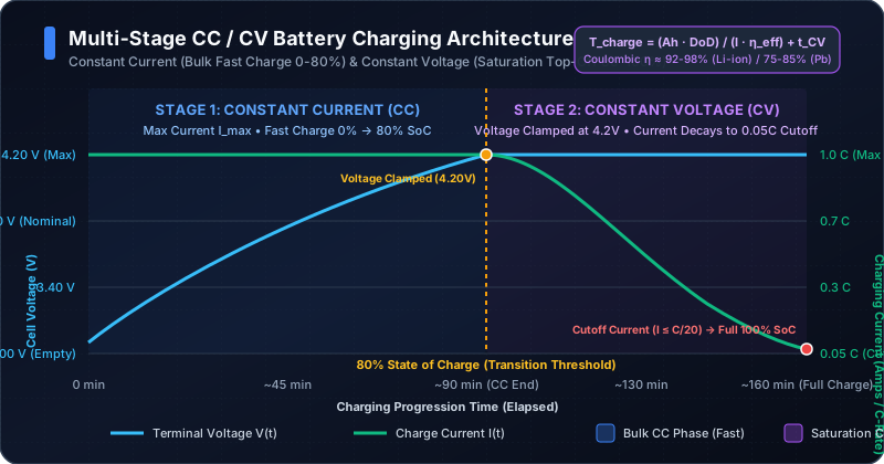
To safely replenish lithium-based and sealed lead-acid chemistries without triggering hazardous thermal runaway or metallic lithium plating, modern chargers employ a two-stage Constant Current / Constant Voltage (CC/CV) algorithmic profile:
- Stage 1: Constant Current (CC) Bulk Fast Charge (0% to ~80% SoC): The charger operates as a regulated current source, pumping the maximum safe continuous current (I_max, typically 0.2C to 0.5C) into the battery. During this phase, cell voltage steadily climbs from its depleted state (e.g. 3.0V) toward its upper electrochemical stabilization voltage (4.20V per cell for lithium-ion NMC, 3.65V for LiFePO4). The CC phase accounts for approximately 75% to 80% of total stored energy and is highly energy-efficient (≈ 95 – 98%).
- Stage 2: Constant Voltage (CV) Saturation Top-Off (80% to 100% SoC): When cell terminal voltage hits the maximum threshold (4.20V), the charger clamps the voltage and transitions into a voltage regulator. Because the open-circuit electrochemical potential of the cell rises to match the charger voltage, the effective driving voltage differential (ΔV = V_charger - V_cell) shrinks, causing charging current to decay exponentially:
The saturation phase takes disproportionately longer than the bulk phase, frequently requiring 1.5 to 2.5 hours to pack in the remaining 20% of capacity. Charging is officially terminated when current drops below a designated cutoff threshold, typically C/20 or 0.05 × I_rated.
3. Time-of-Use (TOU) Electricity Tariffs & Duty-Cycle Optimization
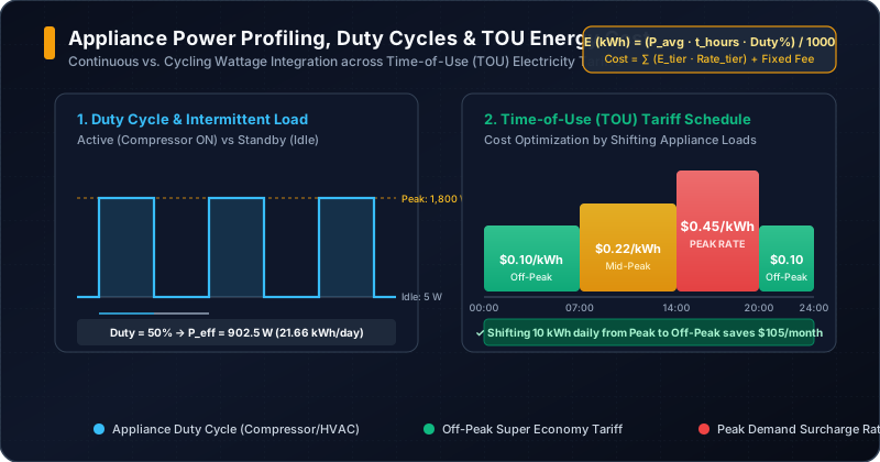
Modern electrical grids face extreme diurnal load imbalances driven by air conditioning spikes and industrial demand between 2:00 PM and 8:00 PM. In response, utilities worldwide have transitioned from archaic flat-rate pricing to dynamic Time-of-Use (TOU) tiered tariffs. Under TOU structures, electricity during peak evening hours can cost 3× to 5× more per kilowatt-hour ($0.45/kWh vs. $0.10/kWh off-peak).
When calculating operational expenditure for high-power residential appliances (such as EV Level 2 home chargers, pool pumps, and electric water heaters), understanding appliance duty cycle (D) is vital:
For example, a 3-ton central air conditioning system with a nameplate draw of 3,500 Watts running 10 hours a day at a 60% compressor duty cycle consumes 3,500 × 10 × 0.60 / 1000 = 21 kWh/day. If programmed to precool the home during off-peak morning hours ($0.12/kWh) rather than peak afternoon hours ($0.42/kWh), household electricity expenses drop by over $189 every month without sacrificing thermal comfort.
4. IoT & Embedded Device Power Profiling
In modern battery-powered wireless sensing applications (e.g. LoRaWAN environmental nodes, Bluetooth Low Energy beacons, and smart agricultural monitors), devices are engineered to survive for 5 to 10 years on a single non-rechargeable lithium cell (Li-SOCl₂ or standard 18650 cell). To achieve this, embedded firmware utilizes extreme duty cycling.
During deep sleep, the microcontroller disables high-frequency crystal oscillators, core ALUs, and RF front-ends, leaving only a micro-power real-time clock (RTC) running. In this quiescent state, current draw drops to a minuscule 5 – 15 μA. Once every 5 or 10 minutes, the device wakes up for 2 to 3 seconds, takes sensor measurements, powers up the radio transceiver (drawing 50 – 100 mA during RF transmission), and immediately returns to deep sleep. The average current is mathematically determined by weighted integration:
With a 99.5% sleep duty ratio, an average current of only 0.05 mA allows a standard 2,500 mAh battery to operate continuously for over 45,000 hours (5.1 years).
5. Wave Propagation Geometry: Acoustic SPL & Photometric Illuminance
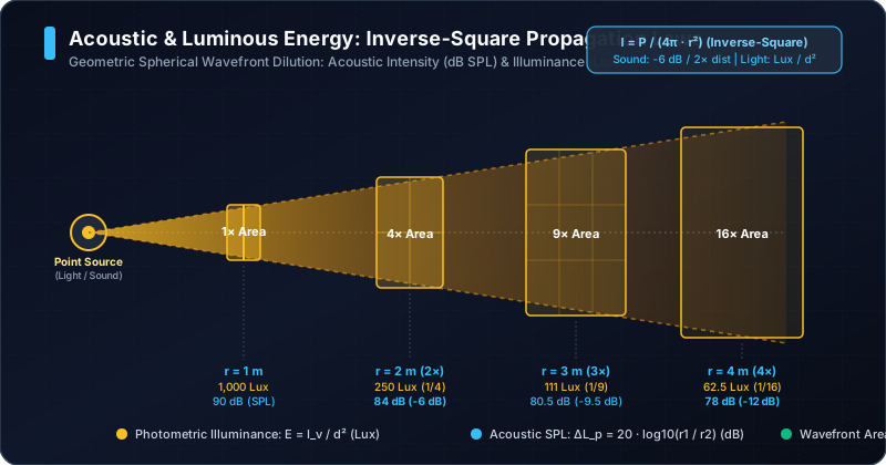
Both acoustic sound waves and optical electromagnetic photons obey the fundamental geometrical Inverse-Square Law when radiating into three-dimensional free space from an isotropic point source. Because total radiated energy spreads evenly across an expanding spherical wavefront whose surface area increases quadratically (A = 4πr²), the flux density (power per unit area) drops proportionally to 1/r².
Acoustic Sound Pressure (dB SPL)
Acoustic intensity I = (P_ac · Q) / (4π · r²) is converted to logarithmic decibels referenced to human hearing threshold (I₀ = 10⁻¹² W/m²). Every doubling of distance reduces sound pressure level by exactly:
Photometric Illuminance (Lux)
Surface illuminance E measures visible light flux received per unit area (1 Lux = 1 lumen/m²). From a directional lamp emitting luminous intensity I_v (candela), illuminance at distance d is: